Printable Chi Square Table / Chi-Square Test of Independence - SPSS Tutorials - LibGuides at Kent State University - Calculators for chi square distribution cgi program by jan de leeuw.
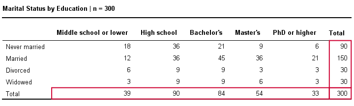
Printable Chi Square Table / Chi-Square Test of Independence - SPSS Tutorials - LibGuides at Kent State University - Calculators for chi square distribution cgi program by jan de leeuw.. , zk are all standard normal random variables (i.e., each zi ~ n (0,1)), and if they are independent, then. Chisq.test(data) following is the description of the parameters used −. Then go to the x axis to find the second decimal number (0.07 in this case). A chi square test of a contingency table helps identify if there are differences between two or more demographics. Find the first two digits on the y axis (0.6 in our example).
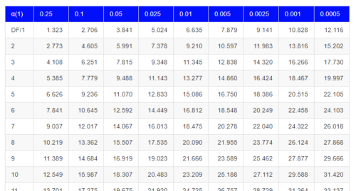
The second page of the table gives chi square values for the left end and the middle of the distribution. Calculators for chi square distribution cgi program by jan de leeuw. Find the first two digits on the y axis (0.6 in our example). The distribution table shows the critical values for chi squared probailities. Data is the data in form of a table containing the count value of the variables in the observation.
Chi Square Statistic Table | Decoration Cloth from spss-tutorials.com The alpha level for the test (common choices are 0.01, 0.05, and 0.10) No cells had an expected count less than 5, so this assumption was met. This means that we use the column corresponding to 0.95 and row 11 to give a critical value of 19.675. Find the first two digits on the y axis (0.6 in our example). And is used in test for the independence of two variables in a contingency table and for tests fir goodness of fit of an observed data to see if it matches to a theoretical one. The second page of the table gives chi square values for the left end and the middle of the distribution. Statistical tables 1 table a.1 cumulative standardized normal distribution a(z) is the integral of the standardized normal distribution from −∞to z (in other words, the area under the curve to the left of z). The footnote for this statistic pertains to the expected cell count assumption (i.e., expected cell counts are all greater than 5):
The distribution table shows the critical values for chi squared probailities.
One of the more confusing things when beginning to study stats is the variety of available test statistics. Javascript program by john walker. .995.99.975.95.9.1.05.025.01 1 0.00 0.00 0.00 0.00 0.02 2.71 3.84 5.02 6.63 2 0.01 0.02 0.05 0.10 0.21 4.61 5.99 7.38 9.21 This means that we use the column corresponding to 0.95 and row 11 to give a critical value of 19.675. To look up an area on the left, subtract it from one, and then look it up (ie: Compute table of expected counts : Calculators for chi square distribution cgi program by jan de leeuw. And is used in test for the independence of two variables in a contingency table and for tests fir goodness of fit of an observed data to see if it matches to a theoretical one. (row total * column total)/ total n for table men (50 * 70) /100 =35 15 50 women 35 15 50 total 70 30 100 compute the chi‐squared statistic: No cells had an expected count less than 5, so this assumption was met. Statistical tables 1 table a.1 cumulative standardized normal distribution a(z) is the integral of the standardized normal distribution from −∞to z (in other words, the area under the curve to the left of z). The value of the test statistic is 3.171. The critical values are calculated from the probability α in column and the degrees of freedom in row of the table.
Find the first two digits on the y axis (0.6 in our example). We can develop a null hypothesis (h0) that point of view and gender are independent and an alternate hypothesis (ha) that gender and point of view are related 0.05 on the left is 0.95 on the right) The value of the test statistic is 3.171. This means that we use the column corresponding to 0.95 and row 11 to give a critical value of 19.675.
6.8 - Chi-square distribution - biostatistics.letgen.org from biostatistics.letgen.org A chi square test of a contingency table helps identify if there are differences between two or more demographics. Finding a corresponding probability is fairly easy. Again, the fis across the top represent 913 Chi square value is 14.067. The first row represents the probability values and the first column represent the degrees of freedom. The critical values are calculated from the probability α in column and the degrees of freedom in row of the table. Calculators for chi square distribution cgi program by jan de leeuw. Then go to the x axis to find the second decimal number (0.07 in this case).
This means that for 7 degrees of freedom, there is exactly 0.05 of the area under the chi square distribution that lies to the right of ´2 = 14:067.
Statistical tables 1 table a.1 cumulative standardized normal distribution a(z) is the integral of the standardized normal distribution from −∞to z (in other words, the area under the curve to the left of z). Df 0.995 0.975 0.20 0.10 0.05 0.025 0.02 0.01 0.005 0.002 0.001; Chi square value is 14.067. , zk are all standard normal random variables (i.e., each zi ~ n (0,1)), and if they are independent, then. 0.05 on the left is 0.95 on the right) The critical values are calculated from the probability α in column and the degrees of freedom in row of the table. Critical values for the chi square distribution The distribution table shows the critical values for chi squared probailities. This means that for 7 degrees of freedom, there is exactly 0.05 of the area under the chi square distribution that lies to the right of ´2 = 14:067. Df 2 f 0.100 2 f 0.050 2 f 0.025 2 0.010 2 0.005 1 2.706 3.841 5.024 6.635 7.879 2 4.605 5.991 7.378 9.210 10.597 A chi square distribution on the other hand, with k degrees of freedom is the distribution of a sum of squares of k independent standard normal variables. Then go to the x axis to find the second decimal number (0.07 in this case). Javascript program by john walker.
The footnote for this statistic pertains to the expected cell count assumption (i.e., expected cell counts are all greater than 5): Find the first two digits on the y axis (0.6 in our example). This means that for 7 degrees of freedom, there is exactly 0.05 of the area under the chi square distribution that lies to the right of ´2 = 14:067. A chi square test of a contingency table helps identify if there are differences between two or more demographics. The areas given across the top are the areas to the right of the critical value.
95 INFO TABLE TEST CHI2 PDF CDR PSD PRINTABLE ZIP - * TableTest from lh5.googleusercontent.com The footnote for this statistic pertains to the expected cell count assumption (i.e., expected cell counts are all greater than 5): To look up an area on the left, subtract it from one, and then look it up (ie: The critical values are calculated from the probability α in column and the degrees of freedom in row of the table. Javascript program by john walker. The value of the test statistic is 3.171. Chisq.test(data) following is the description of the parameters used −. 0.05 on the left is 0.95 on the right) No cells had an expected count less than 5, so this assumption was met.
Critical values for the chi square distribution
A chi square distribution on the other hand, with k degrees of freedom is the distribution of a sum of squares of k independent standard normal variables. The areas given across the top are the areas to the right of the critical value. Critical values for the chi square distribution Compute table of expected counts : Df 0.995 0.975 0.20 0.10 0.05 0.025 0.02 0.01 0.005 0.002 0.001; .995.99.975.95.9.1.05.025.01 1 0.00 0.00 0.00 0.00 0.02 2.71 3.84 5.02 6.63 2 0.01 0.02 0.05 0.10 0.21 4.61 5.99 7.38 9.21 How to use chi squared table? A chi square test of a contingency table helps identify if there are differences between two or more demographics. The footnote for this statistic pertains to the expected cell count assumption (i.e., expected cell counts are all greater than 5): Then go to the x axis to find the second decimal number (0.07 in this case). Finding a corresponding probability is fairly easy. 0.05 on the left is 0.95 on the right) Statistical tables 1 table a.1 cumulative standardized normal distribution a(z) is the integral of the standardized normal distribution from −∞to z (in other words, the area under the curve to the left of z).


0 Komentar